Question 5
Question 7
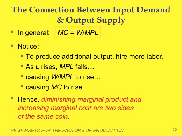
MC = W/MPL
Question 8
Operate if Loss < Fixed Cost
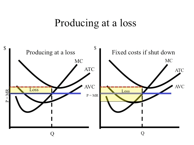
As demonstrated in the table, if the price is below average total cost but above average variable cost, losses are minimized by producing 50 units and incurring a loss of $3.50.
If the firm shut down, it would still have to pay fixed cost of five.
Since average variable costs at 50 units is 42 cents and the price is 45 cents, it covers the variable costs and contributes three cents on each unit toward the paying the fixed costs.
Three cents times 50 units is $1.50 which is the amount the firm has reduced their loss by producing instead of shutting down.
Question 9
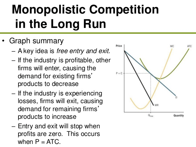
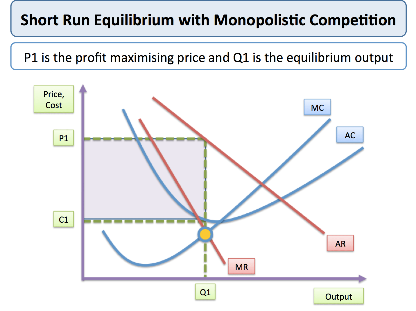
In the long-run the profit for a monopolistically competitive frim is 0
Question 11
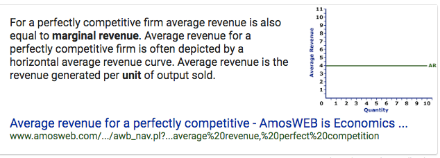
The Marginal Revenue of a firm in a perfectly competitive industry is constant
Question 12
Cost Minimization
Optimal Input Mix is where MPL/Wage = MPK/Rental Rate
If MPL/Wage > MPK/Rental Rate, then hire the human worker
If MPK/Rental Rate > MPL/Wage, then the machines win! use more capital
Question 15
Question 18
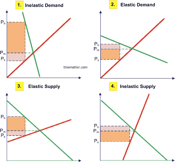
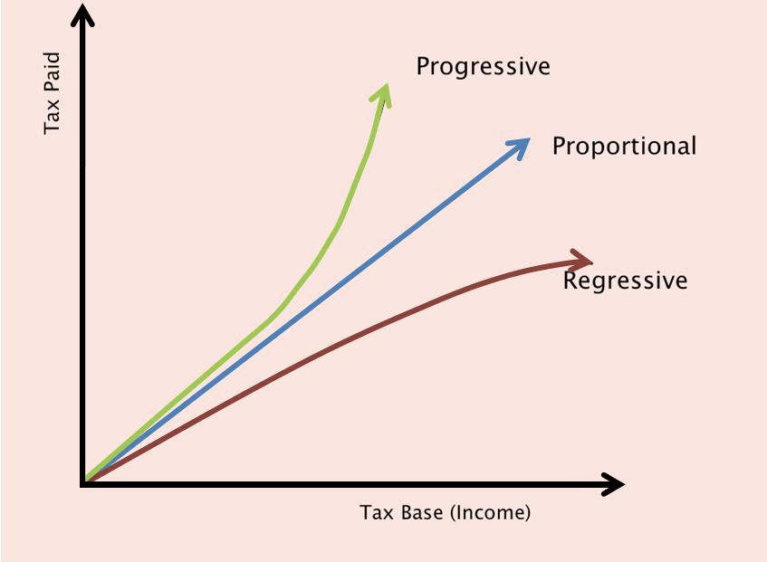
Price elasticity and tax share
Question 19
Question 24
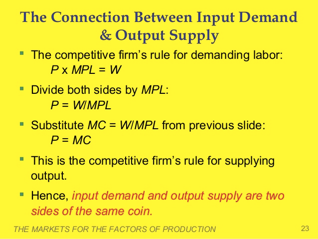
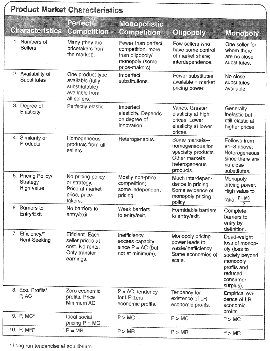
P = MC --> Must be Perfectly Competitive
Question 26
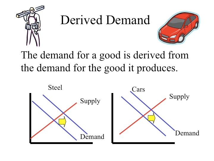
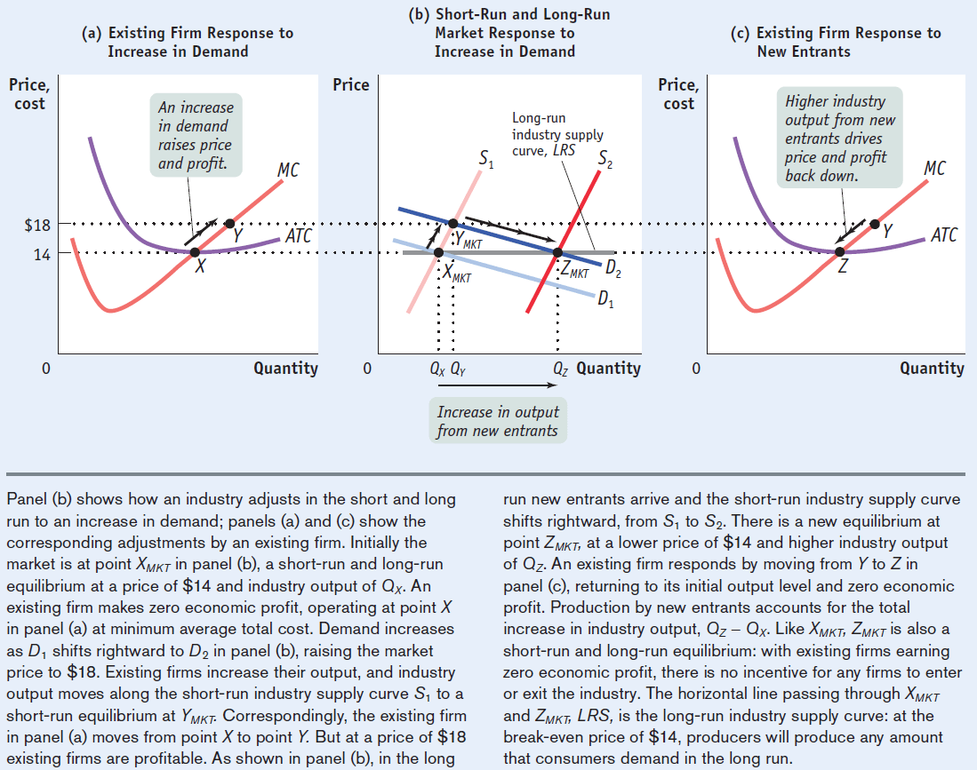
The Effect of an Increase in Demand
An increase in the demand for a product causes the equilibrium price and quantity to increase in the market.
An increase in demand raises price and profit, which causes more suppliers to enter the market
Higher industry output from new entrants drives price and profit back down to its original equilibrium
Question 28
Question 37
For a monopolistically competitive profit-maximizing firm, AR = P
Question 38
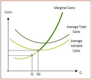
The short-run supply curve for a firm in a perfectly competitive industry is its marginal cost curve above the minimum point of its average variable cost curve
In the short run the firm needs only to cover its variable costs (at Q1 below) – this is largely because covering variable cost ensures than an output can be produced in the future - if variable costs cannot be covered then no further output can be made.
In addition, fixed costs have already been paid for prior to any marginal decision to supply, so do not enter into the firm’s short run calculations.
Question 44
Question 49
Question 51
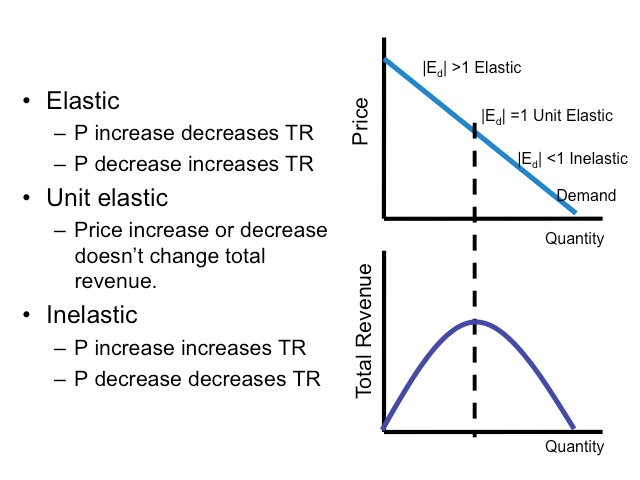
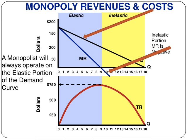
A profit-maximizing monopolist selects its output level in the elastic region of its demand curve.
Question 56